CR, AVE, HTMT: assessing reliability, convergent validity and discriminant validity
Cronbach's Alpha isn't enough to prove a scale is good. This article explains CR, AVE and HTMT with a worked example, cited thresholds and the order to report them in a thesis.
Quick summary
- Outer loadings should be ≥ 0,708; 0,40 to 0,708 are only dropped if that helps CR/AVE pass and the content allows; below 0,40, drop.
- CR = (Σλ)² / [(Σλ)² + Σ(1 − λ²)], ideally 0,70–0,95; 0,60–0,70 is acceptable for exploratory research (Hair et al., 2019).
- AVE = Σλ² / n, needs ≥ 0,50 (Fornell & Larcker, 1981). Example: 4 loadings 0,78; 0,82; 0,75; 0,80 give CR ≈ 0,867 and AVE ≈ 0,621.
- Fornell–Larcker: √AVE must exceed all the construct's correlations, but this criterion detects problems poorly (Henseler et al., 2015).
- HTMT < 0,85 (conservative) or < 0,90 for conceptually close constructs, and the bootstrap confidence interval must not contain 1.
Reliability, convergent validity and discriminant validity
After checking Cronbach's Alpha and exploratory factor analysis, the measurement model (CFA in AMOS or PLS-SEM in SmartPLS) must answer three different questions:
- Reliability: do a scale's questions give consistent results? Indicators: Cronbach's Alpha, rho_A, composite reliability CR.
- Convergent validity: do the questions measure the same construct, and how much of their variance does it explain? Indicators: loadings and AVE.
- Discriminant validity: is this construct really different from the others in the model? Indicators: Fornell–Larcker and HTMT.
A scale can be highly reliable but not distinct: "satisfaction" and "enjoyment" scales may both have high CR while respondents see them as one. So all three groups must be reported. The criteria below apply to reflective scales, not formative ones.
Outer loadings: the starting point
Every indicator here is computed from the standardised loading λ of each observed item (outer loading in SmartPLS, Standardized Regression Weights in AMOS). Hair, Risher et al. (2019) recommend:
| Loading | What to do | Source |
|---|---|---|
| ≥ 0,708 | Keep. The construct explains over 50% of the item's variance (0,7082 ≈ 0,50) | Hair, Risher et al. (2019) |
| 0,40 – 0,708 | Only drop it if that lets CR or AVE pass and doesn't lose content validity | Hair et al. (2022) |
| < 0,40 | Type | Hair et al. (2022) |
A loading of 0,65 isn't automatically "bad". If the scale still passes CR and AVE, keeping the item is usually better than impoverishing the construct's content.
CR, rho_A and AVE formulas with worked examples
Composite reliability CR
Unlike Cronbach's Alpha (which assumes every item contributes equally), CR lets each item have its own loading. Hair, Risher et al. (2019) assess: 0,60–0,70 acceptable in exploratory research; 0,70–0,90 satisfactory to good; 0,95 or above is a concern, since the questions may repeat each other or respondents chose one level for everything. The 0,70 threshold for reliability is also Nunnally & Bernstein's (1994) recommendation.
rho_A
Alpha usually underestimates, and CR overestimates, true reliability. Dijkstra & Henseler (2015) proposed rho_A, which usually lies between the two. SmartPLS 4 calls CR Composite reliability (rho_c) and rho_A Composite reliability (rho_a); don't mix up the two columns when reporting.
Average variance extracted AVE
AVE is the average share of the items' variance explained by the construct. Fornell & Larcker (1981) set AVE ≥ 0,50: the construct explains more variance than measurement error.
| Variable | λ | λ2 | 1 − λ2 |
|---|---|---|---|
| CL1 | 0,78 | 0,6084 | 0,3916 |
| CL2 | 0,82 | 0,6724 | 0,3276 |
| CL3 | 0,75 | 0,5625 | 0,4375 |
| CL4 | 0,80 | 0,6400 | 0,3600 |
| Total | 3,15 | 2,4833 | 1,5167 |
- (Σλ)2 = 3,152 = 9,9225
- CR = 9,9225 / (9,9225 + 1,5167) = 9,9225 / 11,4392 ≈ 0,867, good
- AVE = 2,4833 / 4 ≈ 0,621 ≥ 0,50: convergent validity achieved; √AVE ≈ 0,788
In Excel, with the loadings in B2:B5: CR =SUM(B2:B5)^2/(SUM(B2:B5)^2+SUMPRODUCT(1-B2:B5^2)), AVE =SUMSQ(B2:B5)/COUNT(B2:B5) (some locales use semicolons instead of commas). Don't take loadings from the EFA Pattern Matrix to compute the CR/AVE you report; use loadings from CFA or PLS-SEM.
The Fornell–Larcker criterion
Fornell & Larcker (1981) argue a construct must share more variance with its own items than with any other construct. How to read it: put √AVE on the diagonal of the construct correlation matrix; each diagonal value must exceed every correlation in its row and column.
| Construct | AVE | CL | HL | TT |
|---|---|---|---|---|
| Service quality (CL) | 0,621 | 0,788 | ||
| Satisfaction (HL) | 0,669 | 0,612 | 0,818 | |
| Loyalty (TT) | 0,706 | 0,498 | 0,674 | 0,840 |
In the example, HL's largest correlation is 0,674 (with TT), below the √AVE of HL (0,818) and TT (0,840), so the criterion is met.
HTMT and bootstrap confidence intervals
HTMT (heterotrait-monotrait ratio) compares the correlations between items of two different constructs with the correlations between items within the same construct:
Example: the mean cross-correlation between HL and TT items is 0,494; the mean within-correlation of HL is 0,60, of TT 0,65. HTMT = 0,494 / √(0,60 × 0,65) = 0,494 / 0,6245 ≈ 0,791. An HTMT approaching 1 means the two scales measure almost the same thing.
Thresholds per Henseler et al. (2015): HTMT < 0,85 is conservative; < 0,90 is acceptable for theoretically close constructs (such as satisfaction and loyalty). Beyond the point value, the HTMT bootstrap confidence interval must not contain 1; Hair, Risher et al. (2019) suggest a stricter test against 0,90 or 0,85 depending on context.
| Construct pair | HTMT | 95% confidence interval | Assessment |
|---|---|---|---|
| CL – HL | 0,712 | [0,631; 0,786] | Passed |
| CL – TT | 0,583 | [0,489; 0,672] | Passed |
| HL – TT | 0,791 | [0,718; 0,862] | Passes 0,90; upper bound exceeds 0,85 |
The HL – TT pair passes the 0,85 threshold on the point value and its interval doesn't contain 1, but the upper bound 0,862 exceeds 0,85. Since satisfaction and loyalty are theoretically close, using 0,90 is reasonable; state this argument. In SmartPLS, HTMT is under Calculate → PLS-SEM algorithm → Discriminant validity, with the confidence interval in the results of Calculate → Bootstrapping (how to read bootstrapping: see the article mediators and bootstrapping).
When an indicator fails
- Low AVE or CR: look for items loading below 0,708. Only drop one if it is weak in both numbers and content (vague question, double negative, unrecoded reverse item).
- CR above 0,95: reread the questions; they may be near-duplicates, or respondents may have chosen the same level for everything.
- HTMT cao: look for pairs of questions with overlapping wording across the two scales and items cross-loading strongly on the other construct. Only merge two constructs with a clear theoretical basis, and record it as a model change.
- Don't delete items just to "pass the threshold". Every dropped item needs a reason recorded in the thesis. A scale that passes every indicator but has 2 questions left usually loses content validity.
Common mistakes: reporting only Fornell–Larcker; confusing rho_A with CR; using EFA loadings to compute AVE; applying reflective criteria to formative scales.
Which tool to use for CR, AVE and HTMT
- SPSS has no built-in CR, AVE or HTMT. You can run Alpha and EFA in SPSS, but these indicators must be computed in other tools.
- SmartPLS:
Calculate → PLS-SEM algorithm, xem Construct reliability and validity (Alpha, rho_a, rho_c, AVE) and Discriminant validity (Fornell–Larcker, HTMT). - AMOS: run CFA, take the Standardized Regression Weights table and compute CR and AVE with the formulas above or a plugin. For CFA, Hair, Black et al. (2019) recommend standardised loadings ≥ 0,50, ideally ≥ 0,70.
- By hand / Excel: use the formulas above; HTMT needs the correlation matrix of the observed items.
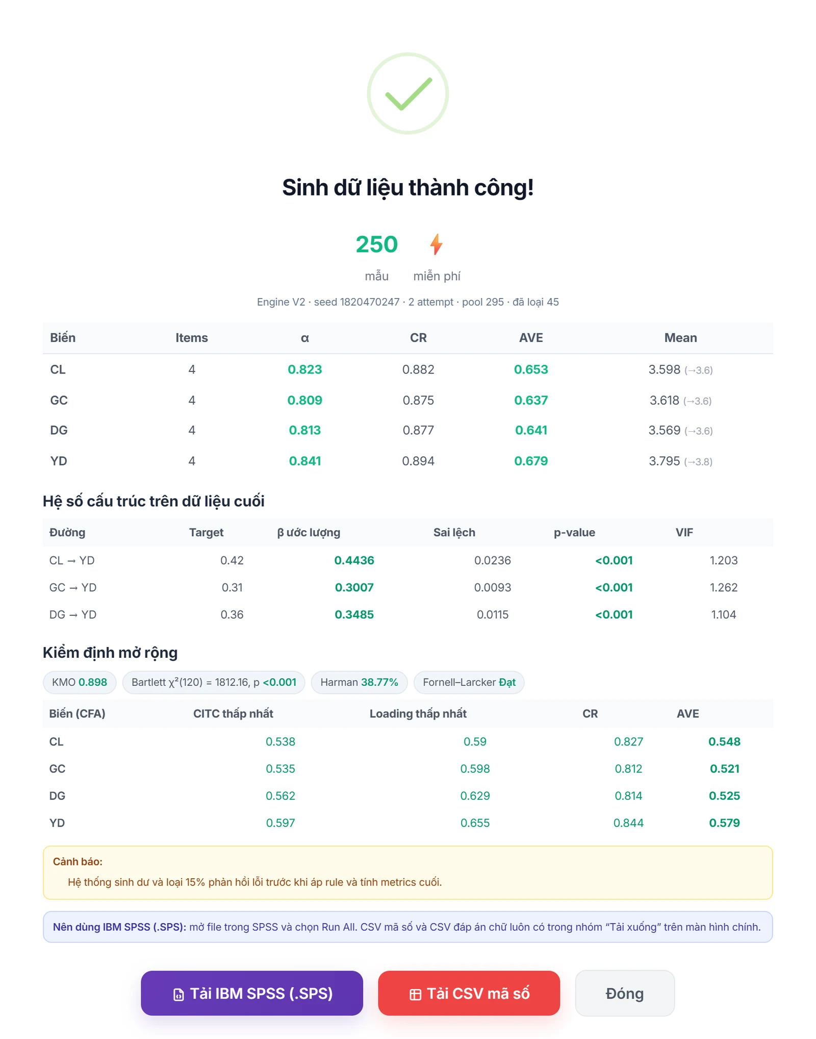
When designing the model, the module AutoFillForm SPSS research computes Alpha, CR, AVE, HTMT and VIF on the current data so you can see how each construct behaves before running SmartPLS. If it is simulated data, only use it to pilot the questionnaire and rehearse the analysis, never instead of real survey data or to polish results.
Reporting order and checklist
In the results chapter, present the measurement model before the structural model, in this order: (1) loadings, Alpha, rho_A, CR, AVE; (2) the Fornell–Larcker table; (3) the HTMT table with confidence intervals.
| Construct | Items | Loading | Alpha | rho_A | CR | AVE |
|---|---|---|---|---|---|---|
| CL | 4 | 0,75 – 0,82 | 0,836 | 0,841 | 0,867 | 0,621 |
| HL | 4 | 0,80 – 0,84 | 0,851 | 0,856 | 0,890 | 0,669 |
| TT | 3 | 0,83 – 0,85 | 0,792 | 0,795 | 0,878 | 0,706 |
Sample conclusion: "All loadings exceed 0,708; CR from 0,867 to 0,890 and AVE from 0,621 to 0,706, meet the thresholds of Hair, Risher et al. (2019) and Fornell & Larcker (1981). All HTMT values are below 0,90 and the 95% bootstrap confidence intervals do not contain 1, so the scales achieve discriminant validity (Henseler et al., 2015)."
- Use standardised loadings from CFA or PLS-SEM, not EFA loadings.
- Loadings ≥ 0,708; items at 0,40–0,708 only dropped with numeric and content reasons.
- CR within 0,70–0,95 and rho_A reported from the right column.
- AVE ≥ 0,50 for every construct.
- HTMT < 0,85 (or < 0,90 with justification) and the bootstrap interval doesn't contain 1.
- Fornell–Larcker is only supplementary, not a replacement for HTMT.
- Every dropped item has a recorded reason.
Frequently asked questions
References
- Fornell, C., & Larcker, D. F. (1981). Evaluating structural equation models with unobservable variables and measurement error. Journal of Marketing Research, 18(1), 39–50.
- Henseler, J., Ringle, C. M., & Sarstedt, M. (2015). A new criterion for assessing discriminant validity in variance-based structural equation modeling. Journal of the Academy of Marketing Science, 43(1), 115–135.
- Hair, J. F., Risher, J. J., Sarstedt, M., & Ringle, C. M. (2019). When to use and how to report the results of PLS-SEM. European Business Review, 31(1), 2–24.
- Hair, J. F., Black, W. C., Babin, B. J., & Anderson, R. E. (2019). Multivariate data analysis (8th ed.). Cengage Learning.
- Hair, J. F., Hult, G. T. M., Ringle, C. M., & Sarstedt, M. (2022). A primer on partial least squares structural equation modeling (PLS-SEM) (3rd ed.). SAGE Publications.
- Dijkstra, T. K., & Henseler, J. (2015). Consistent partial least squares path modeling. MIS Quarterly, 39(2), 297–316.
- Nunnally, J. C., & Bernstein, I. H. (1994). Psychometric theory (3rd ed.). McGraw-Hill.
The thresholds in this article are common conventions in the sources above. Check them against your supervisor's or target journal's requirements.